Extracting Metrics from text using TextDescriptives#
DaCy allows you to use other packages in the spaCy universe as you normally would - just powered by the DaCy models.
The following tutorial shows you how to use DaCy and TextDescriptives to extract a variety of metrics from text. For more information on the metrics that can be extracted, see the TextDescriptives documentation.
Data#
In this tutorial we’ll use TextDescriptives and DaCy, to get a quick overview of the SMS Spam Collection Data Set. The dataset contains 5572 SMS messages categorized as ham or spam.
Note
The estute among you will have noticed that this dataset is not Danish. This tutorial simply want to show how to use DaCy and TextDescriptives together and hopefully inspire you to use the tools on your own (Danish) data.
To start, let’s load a dataset and get a bit familiar with it.
from textdescriptives.utils import load_sms_data

df = load_sms_data()
df.head()
| label | message | |
|---|---|---|
| 0 | ham | Go until jurong point, crazy.. Available only ... |
| 1 | ham | Ok lar... Joking wif u oni... |
| 2 | spam | Free entry in 2 a wkly comp to win FA Cup fina... |
| 3 | ham | U dun say so early hor... U c already then say... |
| 4 | ham | Nah I don't think he goes to usf, he lives aro... |
df["label"].value_counts()
label
ham     4825
spam     747
Name: count, dtype: int64
Adding TextDescriptives components to DaCy#
Adding TextDescriptives components to a DaCy pipeline, follows exactly the same procedure as for any spaCy model. Let’s add the readability and dependency_distance components. Readability is a component that calculates readability metrics, and dependency_distance is a component that calculates the average dependency distance between words in a sentence. This can be seen a measure of sentence complexity.
Because we are using a DaCy model, the dependency_distance component will use the dependency parser from DaCy for its calculations.
import dacy

nlp = dacy.load("small")  # load the latest version of the small model

nlp.add_pipe("textdescriptives/readability")
nlp.add_pipe("textdescriptives/dependency_distance")
Show code cell output
/home/runner/.local/lib/python3.10/site-packages/transformers/utils/generic.py:441: FutureWarning: `torch.utils._pytree._register_pytree_node` is deprecated. Please use `torch.utils._pytree.register_pytree_node` instead.
  _torch_pytree._register_pytree_node(
/home/runner/.local/lib/python3.10/site-packages/transformers/utils/generic.py:309: FutureWarning: `torch.utils._pytree._register_pytree_node` is deprecated. Please use `torch.utils._pytree.register_pytree_node` instead.
  _torch_pytree._register_pytree_node(
/home/runner/.local/lib/python3.10/site-packages/spacy/util.py:910: UserWarning: [W095] Model 'da_dacy_small_trf' (0.2.0) was trained with spaCy v3.5.2 and may not be 100% compatible with the current version (3.7.5). If you see errors or degraded performance, download a newer compatible model or retrain your custom model with the current spaCy version. For more details and available updates, run: python -m spacy validate
  warnings.warn(warn_msg)
/home/runner/.local/lib/python3.10/site-packages/spacy/util.py:910: UserWarning: [W095] Model 'da_dacy_small_ner_fine_grained' (0.1.0) was trained with spaCy v3.5.0 and may not be 100% compatible with the current version (3.7.5). If you see errors or degraded performance, download a newer compatible model or retrain your custom model with the current spaCy version. For more details and available updates, run: python -m spacy validate
  warnings.warn(warn_msg)
/home/runner/.local/lib/python3.10/site-packages/transformers/utils/generic.py:309: FutureWarning: `torch.utils._pytree._register_pytree_node` is deprecated. Please use `torch.utils._pytree.register_pytree_node` instead.
  _torch_pytree._register_pytree_node(
/home/runner/.local/lib/python3.10/site-packages/spacy_transformers/layers/hf_shim.py:124: FutureWarning: You are using `torch.load` with `weights_only=False` (the current default value), which uses the default pickle module implicitly. It is possible to construct malicious pickle data which will execute arbitrary code during unpickling (See https://github.com/pytorch/pytorch/blob/main/SECURITY.md#untrusted-models for more details). In a future release, the default value for `weights_only` will be flipped to `True`. This limits the functions that could be executed during unpickling. Arbitrary objects will no longer be allowed to be loaded via this mode unless they are explicitly allowlisted by the user via `torch.serialization.add_safe_globals`. We recommend you start setting `weights_only=True` for any use case where you don't have full control of the loaded file. Please open an issue on GitHub for any issues related to this experimental feature.
  self._model.load_state_dict(torch.load(filelike, map_location=device))
/home/runner/.local/lib/python3.10/site-packages/spacy_transformers/layers/hf_shim.py:137: UserWarning: Error loading saved torch state_dict with strict=True, likely due to differences between 'transformers' versions. Attempting to load with strict=False as a fallback...

If you see errors or degraded performance, download a newer compatible model or retrain your custom model with the current 'transformers' and 'spacy-transformers' versions. For more details and available updates, run: python -m spacy validate
  warnings.warn(warn_msg)
/home/runner/.local/lib/python3.10/site-packages/spacy_transformers/layers/hf_shim.py:139: FutureWarning: You are using `torch.load` with `weights_only=False` (the current default value), which uses the default pickle module implicitly. It is possible to construct malicious pickle data which will execute arbitrary code during unpickling (See https://github.com/pytorch/pytorch/blob/main/SECURITY.md#untrusted-models for more details). In a future release, the default value for `weights_only` will be flipped to `True`. This limits the functions that could be executed during unpickling. Arbitrary objects will no longer be allowed to be loaded via this mode unless they are explicitly allowlisted by the user via `torch.serialization.add_safe_globals`. We recommend you start setting `weights_only=True` for any use case where you don't have full control of the loaded file. Please open an issue on GitHub for any issues related to this experimental feature.
  b = torch.load(filelike, map_location=device)
/home/runner/.local/lib/python3.10/site-packages/thinc/shims/pytorch.py:253: FutureWarning: You are using `torch.load` with `weights_only=False` (the current default value), which uses the default pickle module implicitly. It is possible to construct malicious pickle data which will execute arbitrary code during unpickling (See https://github.com/pytorch/pytorch/blob/main/SECURITY.md#untrusted-models for more details). In a future release, the default value for `weights_only` will be flipped to `True`. This limits the functions that could be executed during unpickling. Arbitrary objects will no longer be allowed to be loaded via this mode unless they are explicitly allowlisted by the user via `torch.serialization.add_safe_globals`. We recommend you start setting `weights_only=True` for any use case where you don't have full control of the loaded file. Please open an issue on GitHub for any issues related to this experimental feature.
  model.load_state_dict(torch.load(filelike, map_location=device))
<textdescriptives.components.dependency_distance.DependencyDistance at 0x7f0940188c70>
From now on, whenever we pass a document through the pipeline (nlp), TextDescriptives will add readability and dependency distance metrics to the document.
Let’s load the data and pass it through the pipeline.
# to speed things up (especially on cpu) let's subsample the data
df = df.sample(500)

doc = nlp.pipe(df["message"])
import textdescriptives as td

# extract the metrics as a dataframe
metrics = td.extract_df(doc, include_text=False)
Show code cell output
Token indices sequence length is longer than the specified maximum sequence length for this model (156 > 128). Running this sequence through the model will result in indexing errors
/home/runner/.local/lib/python3.10/site-packages/thinc/shims/pytorch.py:114: FutureWarning: `torch.cuda.amp.autocast(args...)` is deprecated. Please use `torch.amp.autocast('cuda', args...)` instead.
  with torch.cuda.amp.autocast(self._mixed_precision):
/home/runner/.local/lib/python3.10/site-packages/thinc/shims/pytorch.py:114: FutureWarning: `torch.cuda.amp.autocast(args...)` is deprecated. Please use `torch.amp.autocast('cuda', args...)` instead.
  with torch.cuda.amp.autocast(self._mixed_precision):
# join the metrics to the original dataframe
df = df.join(metrics, how="left")
df.head()
| label | message | dependency_distance_mean | dependency_distance_std | prop_adjacent_dependency_relation_mean | prop_adjacent_dependency_relation_std | flesch_reading_ease | flesch_kincaid_grade | smog | gunning_fog | ... | sentence_length_median | sentence_length_std | syllables_per_token_mean | syllables_per_token_median | syllables_per_token_std | n_tokens | n_unique_tokens | proportion_unique_tokens | n_characters | n_sentences | |
|---|---|---|---|---|---|---|---|---|---|---|---|---|---|---|---|---|---|---|---|---|---|
| 3266 | ham | Ok then i come n pick u at engin? | NaN | NaN | NaN | NaN | NaN | NaN | NaN | NaN | ... | NaN | NaN | NaN | NaN | NaN | NaN | NaN | NaN | NaN | NaN |
| 71 | ham | Finished class where are you. | 2.0 | 0.0 | 0.454545 | 0.0 | 64.924545 | 6.936364 | NaN | 11.672727 | ... | 11.0 | 0.0 | 1.545455 | 1.0 | 0.78203 | 11.0 | 11.0 | 1.0 | 45.0 | 1.0 |
| 1915 | ham | Its not that time of the month nor mid of the ... | NaN | NaN | NaN | NaN | NaN | NaN | NaN | NaN | ... | NaN | NaN | NaN | NaN | NaN | NaN | NaN | NaN | NaN | NaN |
| 1324 | ham | Can you call me plz. Your number shows out of ... | NaN | NaN | NaN | NaN | NaN | NaN | NaN | NaN | ... | NaN | NaN | NaN | NaN | NaN | NaN | NaN | NaN | NaN | NaN |
| 5339 | ham | You'd like that wouldn't you? Jerk! | NaN | NaN | NaN | NaN | NaN | NaN | NaN | NaN | ... | NaN | NaN | NaN | NaN | NaN | NaN | NaN | NaN | NaN | NaN |
5 rows × 28 columns
That’s it! Let’s do a bit of exploratory data analysis to get to know the data a bit more.
Exploratory Data Analysis#
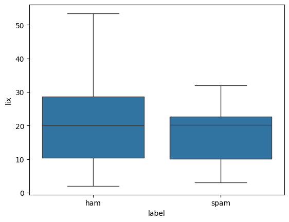
With the metrics extracted, let’s do some quick exploratory data analysis to get a sense of the data. Let us start of by taking a look at the distribution of the readability metrics, lix.
import seaborn as sns

sns.boxplot(x="label", y="lix", data=df)
<Axes: xlabel='label', ylabel='lix'>
Let’s run a quick test to see if any of our metrics correlate strongly with the label
# encode the label as a boolean
df["is_ham"] = df["label"] == "ham"
# compute the correlation between all metrics and the label
metrics_correlations = metrics.corrwith(df["is_ham"]).sort_values(
    key=abs, ascending=False
)
metrics_correlations[:10]
smog                                     -0.499689
n_characters                             -0.275878
sentence_length_std                      -0.249043
n_tokens                                 -0.231495
n_unique_tokens                          -0.220204
token_length_median                      -0.200472
prop_adjacent_dependency_relation_mean   -0.184031
proportion_unique_tokens                  0.167268
coleman_liau_index                       -0.161663
token_length_mean                        -0.147740
dtype: float64
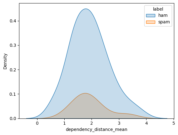
That’s some pretty high correlations! Notably we see that the mean dependency distance is correlated with ham. This makes sense, as the dependency distance is a measure of sentence complexity, and spam messages tend to be shorter and simpler.
Let’s try to plot it:
sns.kdeplot(df, x="dependency_distance_mean", hue="label", fill=True)
<Axes: xlabel='dependency_distance_mean', ylabel='Density'>
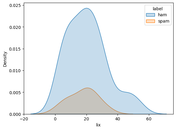
We can do a similar thing for the lix score, where we see that here isn’t a big difference between the two classes:
sns.kdeplot(df, x="lix", hue="label", fill=True)
<Axes: xlabel='lix', ylabel='Density'>
Cool! We’ve now done a quick analysis of the SMS dataset and found some differences in the distributions of some readability and dependency-distance metrics between the actual SMS’s and spam.
Next steps could be continue the exploratory data analysis or to build a simple classifier using the extracted metrics.